How to Pass the Databricks Data Analyst Associate Exam

It was my birthday over the weekend and whilst my body was completely destroyed by whiskey and vermouth… my mind craved sustenance and my soul penance. Therefore I looked at the preparation guidelines for the databricks analyst associate certification and thought “we got this!”. Within 48 hours my mind was full to the brim, my soul ready to redeem some of the reprehensible activities of the weekend by passing the exam and then sharing this approach with you. Here goes…

• Pre-Requisites
• Useful Links
• Analytic Definitions
• Provision Workspace and Unity Catalog
  • Create Workspace
  • Create Storage Account
  • Create Containers
  • Create External Connector \& Grant Access
  • Create Unity Catalog
  • Create External Location
  • Unity Catalog Overview
• Quick SQL Tour and Warehouse Setup
• Create a Folder to Store your Work
• Create Catalog and Schema
• Quick Table Create
• Describe, Time Travel \& Restores
• Managed Tables vs UnManaged Tables
• Import Data
• Minimum SQL
  • Select
  • Subquery and CTE
  • Join
    • Inner Join
    • Left Join
    • Right Join
  • Aggregations and Group by
  • Transform Arrays
  • Merge
• Query History
• Visualisations
• Parameters
• Dashboard
• Alerts
• Book the Exam

Pre-Requisites

• Azure Account - The community edition of databricks doesn’t have the SQL tools of databricks so you’re going to either need to leverage one already provided for you, or create your own in Azure, AWS or Google. I predominantly use Microsoft Azure which is why I have recommended this tooling here. We’ll go through a quick setup of a bare minimum databricks workspace and unity catalog provisioning on Azure anyway just in case you have nowhere to work in.

Useful Links

• Databricks Academy - Sign up to this learning resource which is absolutely free. I actually did the lakehouse fundamentals course first (about 2 hours with speed ramped up) and then do the data analyst learning plan. It says 7 hours but you can do it in much less.
• Kryterion Certification Login - This is where you can book your exam. I booked this 90 minutes before deciding to do this particular exam as I was pretty confident immediately after doing the course above and what I had read about it.
• Udemy Practice Questions. There is no practice exam for the databricks data analyst associate so I thought I would try this Udemy version. I’ll be honest it gave me confidence but a lot of the questions I did not trust or were worded weirdly, so I think I could have done without and kept the ten quid. I believe the below and the databricks academy course should be enough to steer you through.

Disclaimer! I have been using databricks for about 3 years and so knew a fair about the SQL analyst aspects of it. However, I still believe the exam was very straight forward and simply doing the above along with my tips below will easily allow you to pass.

Analytic Definitions

There are a couple of analytic definitions you need to be aware of which are covered below.

• Medallion Architecture: This refers to the bronze, silver and gold layers in a delta lake implementation.
• Bronze Layer - The bronze layer is where raw data lands untouched.
• Silver Layer - This is the data that has been cleansed, deduplicated and missing values handled.
• Gold Layer - This is the layer typically used for analysis as it has been aggregated and optimised for querying.
• Categorical Data : This is data that can be identified based on categorical labels such as place or colour.
• Continuous Data : Continuous data does not have fixed values and can potentially have an infinite number of possible values. It is usually numerical.
• Last Mile ETL : This is data transformation that tends to happen towards the end of a project that is suddenly required and tens to occur on gold tables by analysts.
• Data Blending : This is where two datasets are joined together where there combination is required for further insights.
• Data Enhancement : Data enhancements can be where analysts can add further aggregations or properties to their gold layer queries that provide further information.

Provision Workspace and Unity Catalog

The following section is not needed for the exam but I have put in case you need a workspace to practice your analytics in if you do not have one available. It takes about 15 minutes and is not a bad exercise to understand the workings of it all anyway. The process here is manual but there are ways of automating this using tools such as terraform. This is all out of scope for the exam so just to get what you need for an environment to work within, the following should do. If you already have a workspace and catalog setup skip to Quick SQL Tour and Warehouse Setup.

Create Workspace

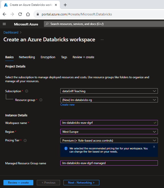
1. Navigate to azure and create a databricks workspace resource using this link.
2. Choose the appropriate subscription.
3. Create a new resource group called lrn-databricks-rg.
4. Name the workspace something appropriate and unique such as lrn-databricks-euw-dgrf (change the last 4 characters to something suitable to yourself).
5. Choose the region (I am using west europe which is also reflected in the workspace name above as “euw”).
6. We’ll have to choose premium so that we can leverage the tooling we want for these exercises and to use unity catalog.
7. Set the managed resource group name to be the same as your resource group name plus “managed”, e.g. lrn-databricks-euw-dgrf-managed.
8. You don’t need to worry about any other options for this so just click review and create. Creating the workspace might take a few minutes.

Create Storage Account

You’ll need to create a storage account to back your unity catalog storage created in the next section so your data can be stored.

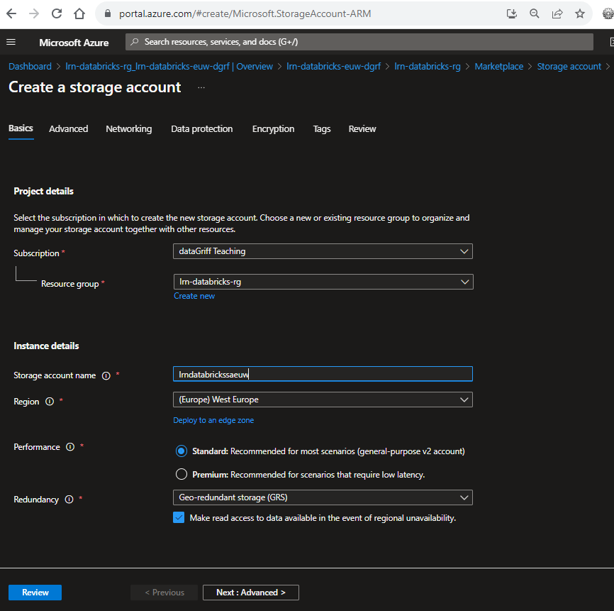
1. Navigate to azure and create a storage account resource using this link.
2. Choose the subscription you created your databricks workspace in.
3. Set the resource group to be the same one you created your workspace in.
4. Set the storage account name to be something like lrncatalogsaeuwdgrf, changing the last four characters to be something unique for your resource.
5. Set the region to be the same as your databricks workspace and the same as the shortcode you placed for the storage - in this case I used West Europe (euw).
6. On the advanced tab ensure that “Enable Hierarchical Namespace” is ticked. This ensures a data lake storage account is created.
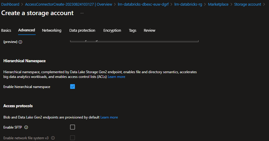
7. Leave everything else the same and select review then create.

Create Containers

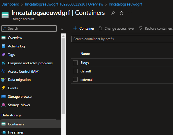
1. Navigate to your storage account in Azure.
2. Click + Container and call it default. This will be used as the default storage container for unity catalog in the next section.
3. Click + Container and call it external. This will be used as container storage for an external location in unity catalog.

Create External Connector & Grant Access

The external connector is how your databricks workspace will authenticate against the storage created above. Permissions for users can then handled by unity catalog whilst all storage permissions are handled by the external connector.

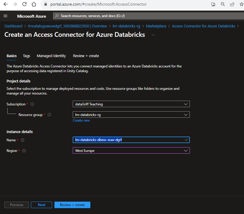
1. Navigate to azure and create a databricks external connector resource using this link.
2. Choose the same subscription you created your other resources in.
3. Choose the same lrn-databricks-rg resource group.
4. Name it something like lrn-databricks-dbexc-euw-dgrf but change the last four characters to make it unique to your resource.
5. Choose the same region that you created your your other resources, for me this was West Europe.
6. Click review and create.
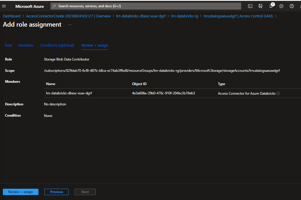
7. Navigate to your storage account, go to Access Control and select + Add.
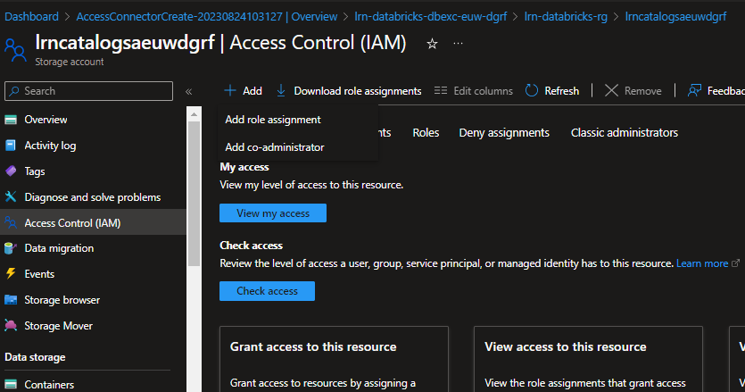
8. For the role choose storage Blob Data Contributor.
9. For members choose Managed Identity, select members and then pick the databricks access connector we have created.
10. Select review and assign.

Create Unity Catalog

1. Launch your new databricks workspace.

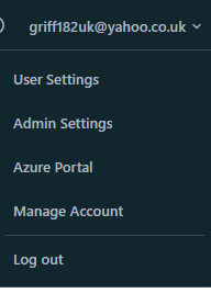
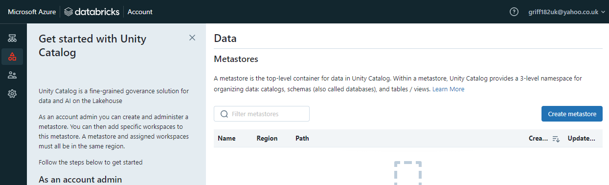
2. In the top right click your user name and navigate to “Manage Account”.

   

3. Choose data and then select “create metastore”.
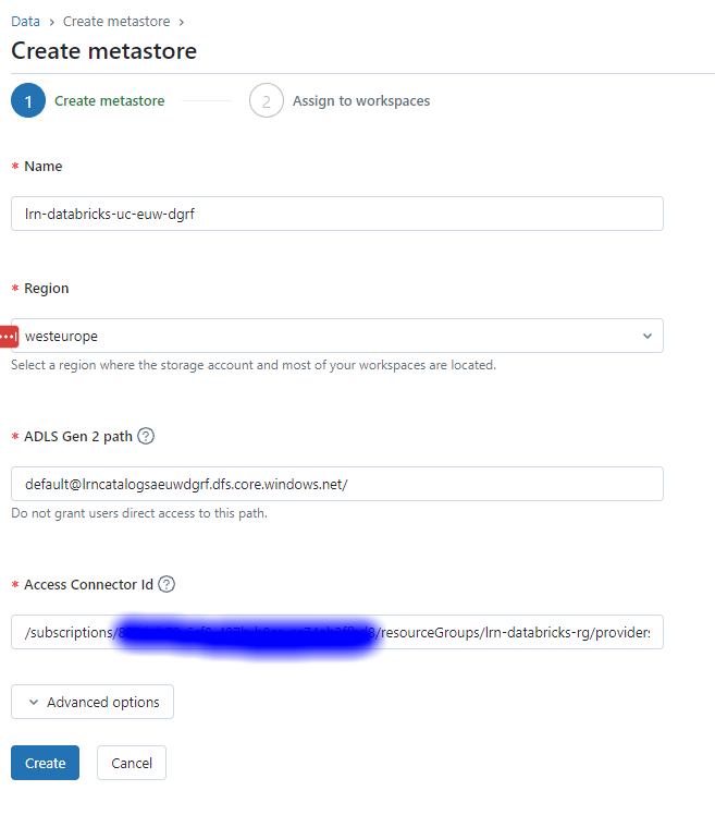
4. Name the metastore lrn-databricks-uc-euw-dgrf, remembering to change the last four characters to something unique to you.
5. Select the same region you created your other resources, in my case it was West Europe again.
6. Set the ADLS Gen 2 Path to be your storage account path which should be something like this: abfss://default@lrncatalogsaeuwdgrf.dfs.core.windows.net/

7. Set the access connector id to be the external connector resource id you created which will be something like this: /subscriptions/xxxxxx-xxxxxx-xxxxxx-xxxxxx-xxxxxx/resourceGroups/lrn-databricks-rg/providers/Microsoft.Databricks/accessConnectors/lrn-databricks-dbexc-euw-dgrf.

   

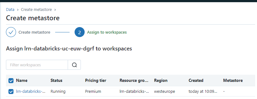
8. Assign the metastore to your new workspace.

Create External Location

External locations are handy if we want to distribute our storage across multiple containers, or even multiple storage accounts for example to manage costs better. To create an external location on the external container we created earlier…

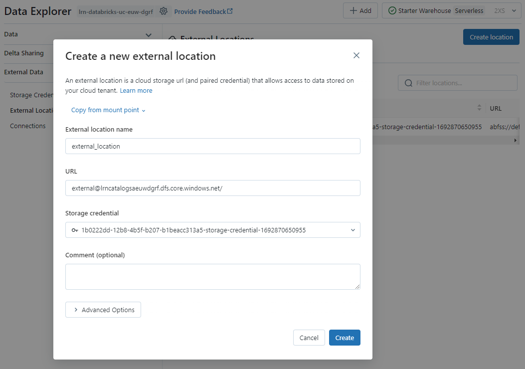
1. Navigate to external data in your workspace.
2. Select “Create Location”.
3. Call it external_location.
4. Set the URL to be abfss://external@lrncatalogsaeuwdgrf.dfs.core.windows.net/, changing the name of the storage to be whatever you created.
5. Set the only storage credential available which will be the external connector already created.

Unity Catalog Overview

Before we carry on, it’s quickly worth noting the unity catalog hierarchy and how it maps to the three part naming conventions we’ll use in our data objects.

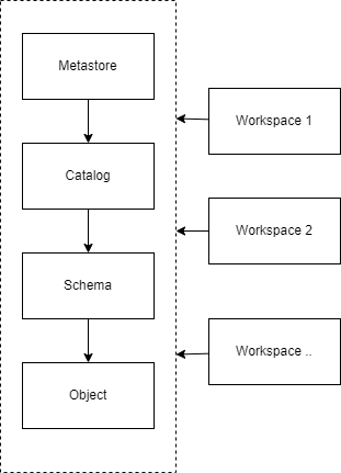
The metastore exists outside the workspaces which allows for multiple workspaces to access the same unity catalog. This means all the objects can be shared between multiple workspaces, even though for this exercise we are only assigning one, we could assign more.

Based on the hierarchy of unity catalog the three part naming components of data objects in are:

• catalog.schema.objectname

Where object name could be a table or a view.

Quick SQL Tour and Warehouse Setup

For the data analyst associate we’re going to be interested in this section of the workspace covering queries, dashboards, alerts, history and warehouses.

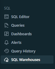
In order to save the pennies, speed up our queries, and to leverage the serverless aspect of databricks that is now available, first go into SQL Warehouses.

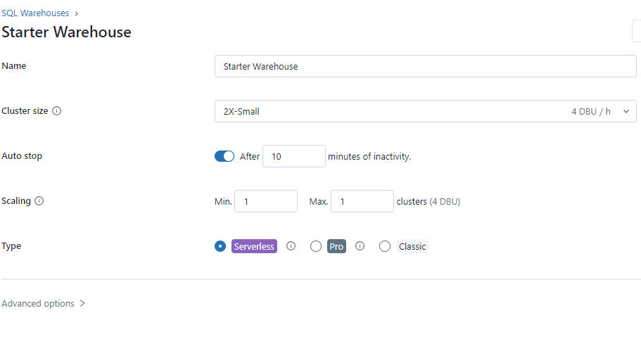
• Select the starter warehouse.
• Click edit.
• Set the cluster size to 2X-Small.
• Set to auto-stop after 10 minutes of inactivity.
• Set the type to be serverless.
• Click save.
• Start the warehouse.

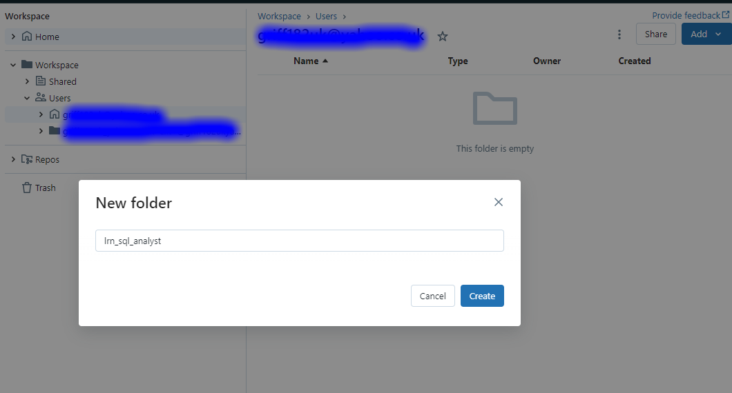
Create a Folder to Store your Work

Before we start creating queries, dashboards and visualisations left, right and centre, lets create a folder to store all this work in. Navigate to workspace, your username, then click add folder. Call the new folder lrn_sql_analyst.

Create Catalog and Schema

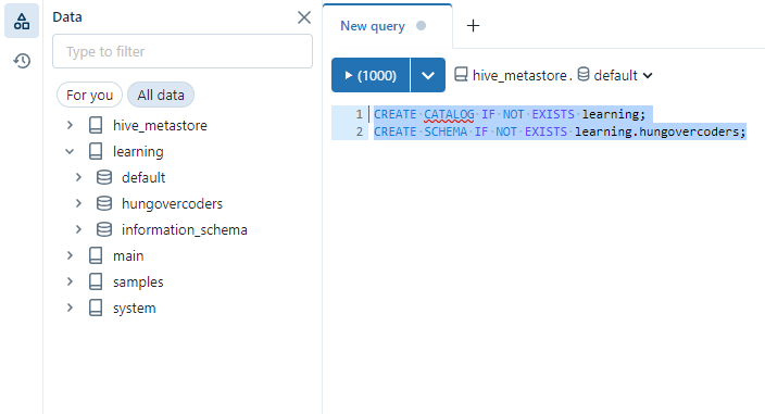
We’re now going to create a catalog and a schema to register our data products in. Navigate to SQL editor in the left hand pane, enter the following code and execute.

CREATE CATALOG IF NOT EXISTS learning;
COMMENT ON CATALOG learning IS 'This catalog is for learning';
CREATE SCHEMA IF NOT EXISTS learning.hungovercoders;
COMMENT ON SCHEMA learning.hungovercoders IS 'This catalog is for hungovercoders material';

You should see a new catalog appear in data and a new schema. Both of these will also have comments on them in data explorer.

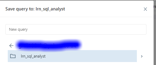
Save the query as “Setup Catalog” in your folder lrn_sql_analyst.

Quick Table Create

At this point lets create a basic table and insert some data. Run the following command in a new query.

CREATE TABLE IF NOT EXISTS learning.hungovercoders.beers
(
  name string,
  brewery string
);

COMMENT ON TABLE learning.hungovercoders.beers IS 'This table containers beers'

INSERT INTO learning.hungovercoders.beers
(
  name, brewery
)
VALUES ('Yawn','Flowerhorn'),('Stay Puft','Tiny Rebel');

SELECT * FROM learning.hungovercoders.beers;

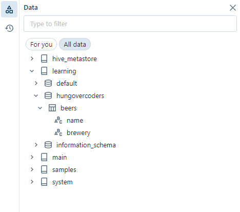
You should the above returns two rows of the two two beers we inserted. Save the query as “Beers” in your lrn_sql_analyst location.

Navigate to data explorer and you’ll also see the table existing there.

If you then open the table in data explorer by clicking the ellipsis next to its name, you will see the comments, columns, sample data, the owner and popularity.

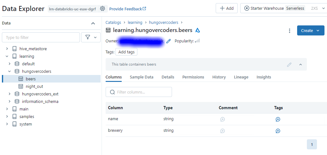
Its worth noting at this point in details you will see that the data is automatically saved in the default container of our unity catalog storage.

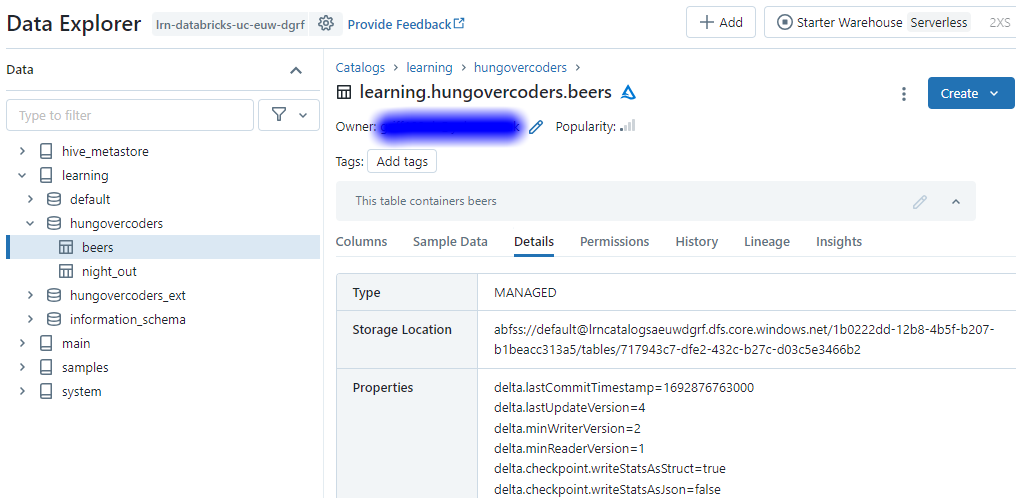
This is because we have not set a location as part of our schema setup so it uses the default. We can create a schema that leverages the external location we created earlier by running the following.

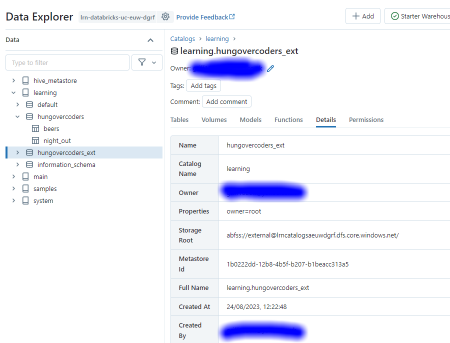
CREATE SCHEMA IF NOT EXISTS learning.hungovercoders_ext MANAGED LOCATION 'abfss://external@lrncatalogsaeuwdgrf.dfs.core.windows.net/';
COMMENT ON SCHEMA learning.hungovercoders IS 'This catalog is for hungovercoders material in an external location';

Save the query as Create External Schema in our lrn_sql_analyst folder. If you now navigate to this schema in data explorer and check details you will see that its using the external location we setup.

Describe, Time Travel & Restores

Create a new query and call it time travel, saving it in the lrn_sql_analyst location. Then run the following query:

DESCRIBE EXTENDED learning.hungovercoders.beers;

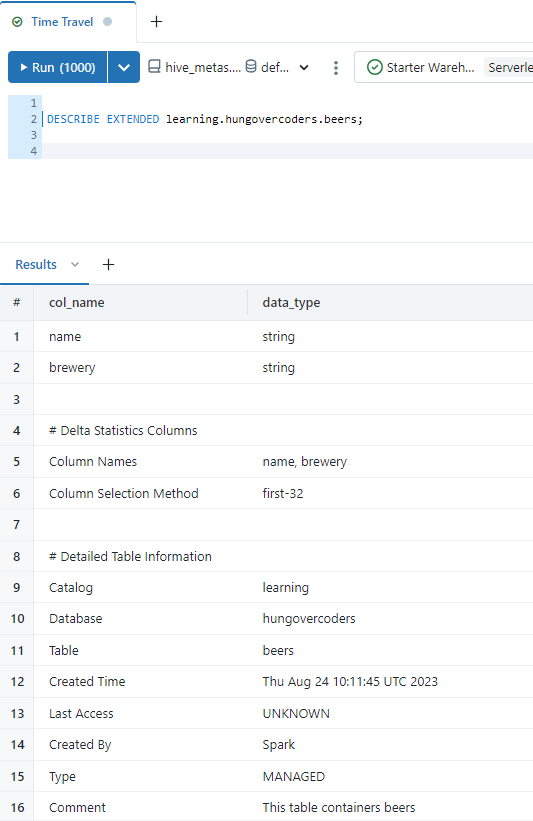
This will give us a lot of information about the table such as whether its managed or unmanaged, the storage location, who created it and the schema.

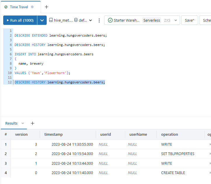
Now if we run the following we can get the version history of the table which includes all the different commits. The ones shown so far will be the creation of the table and writes we have performed against it.

DESCRIBE HISTORY learning.hungovercoders.beers;

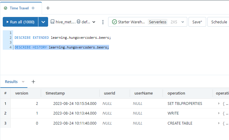
Lets accidentally insert a new duplicate row then look at the history again. We wil now see a new WRITE version in the history based on the new row we inserted in a transaction.

INSERT INTO learning.hungovercoders.beers
(
  name, brewery
)
VALUES ('Yawn','Flowerhorn');
DESCRIBE HISTORY learning.hungovercoders.beers;

If we want to query a previous version we can run this command.

SELECT * FROM learning.hungovercoders.beers VERSION AS OF 1;

If we want to completely restore the table to a previous we can run this command.

RESTORE learning.hungovercoders.beers VERSION AS OF 1;

Managed Tables vs UnManaged Tables

A managed table couples the pointer in unity catalog and the data so that when the table is dropped the data is also dropped. An unmanaged table does not couple the table metadata object and the data so that when the table is dropped the data is not dropped as well. We have only made managed tables so far therefore any table we actually drop will remove the data as well.

Import Data

First we need to download some sample data. Download this file to your local machine which is a simple csv of locations and what was drank.

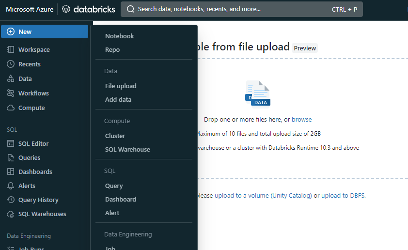
To import data easily into databricks (up to 1GB in size), select + New on the left hand side of the workspace and choose “File Upload”.

Navigate to the file you just downloaded and select it to import. Change the catalog to be learning, the schema to be hungovercoders and call the table “night_out”. Your screen should look something like the below.

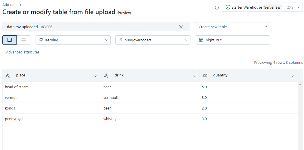
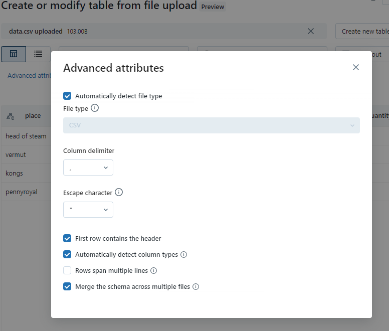
You can make changes on the data types if you wish by clicking the icons next to the column names and also Under advanced attributes you can also make changes there such as the delimiter, and whether the rows contain a header.

We’re happy with our little table though so we can select Create Table.

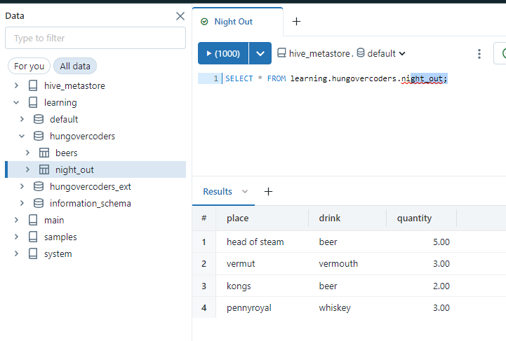
Now if we go back to SQL Editor and create a new query called “Night Out” and save it in the lrn_sql_analyst location. We can now run the below and interact with the data we just uploaded like a normal table.

Minimum SQL

The following should give the minimum amount of commands you’re going to need to know for the exam… Lets go!

Select

Create a query and name it “Select”, saving in the lrn_sql_analyst location. Enter the following, save and we can see the mighty SELECT is how we get data from a table.

SELECT * FROM learning.hungovercoders.night_out;

Subquery and CTE

Create a query and name it “Subqueries & CTEs”, saving in the lrn_sql_analyst location. A subquery is how we can perform small queries with a SELECT statement that we can reference say as part of a join.

SELECT
  night.place,
  night.drink,
  ref.type,
  night.quantity
FROM
  learning.hungovercoders.night_out night
  JOIN (
    SELECT
      'head of steam' AS place,
      'pub' AS type
    UNION ALL
    SELECT
      'vermut' AS place,
      'bar' AS type
    UNION ALL
    SELECT
      'kongs' AS place,
      'bar' AS type
    UNION ALL
    SELECT
      'pennyroyal' AS place,
      'pub' AS type
  ) AS ref on ref.place = night.place

We can make these easier to manage by encapsulating them in common table expressions at the start of a query and just reference that.

WITH CTE_ref AS
(
  SELECT
      'head of steam' AS place,
      'pub' AS type
    UNION ALL
    SELECT
      'vermut' AS place,
      'bar' AS type
    UNION ALL
    SELECT
      'kongs' AS place,
      'bar' AS type
    UNION ALL
    SELECT
      'pennyroyal' AS place,
      'pub' AS type
)
SELECT
  night.place,
  night.drink,
  ref.type,
  night.quantity
FROM
  learning.hungovercoders.night_out night
  JOIN CTE_ref AS ref on ref.place = night.place

Join

Joins are how we can link tables together and bring them back in a single output. The three joins we’ll look at here are inner, left and right joins.

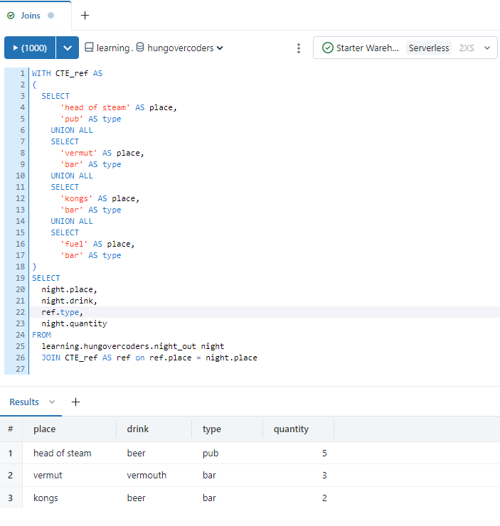
Inner Join

Create a query and name it “Joins”, saving in the lrn_sql_analyst location. Run the following command we will only get three results returned because the reference data does not contain pennyroyal and the night out table does not contain fuel. The inner join means that rows that exist in both tables only will be returned.

WITH CTE_ref AS
(
  SELECT
      'head of steam' AS place,
      'pub' AS type
    UNION ALL
    SELECT
      'vermut' AS place,
      'bar' AS type
    UNION ALL
    SELECT
      'kongs' AS place,
      'bar' AS type
    UNION ALL
    SELECT
      'fuel' AS place,
      'bar' AS type
)
SELECT
  night.place,
  night.drink,
  ref.type,
  night.quantity
FROM
  learning.hungovercoders.night_out night
  JOIN CTE_ref AS ref on ref.place = night.place

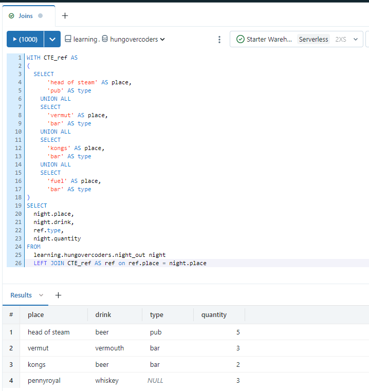
Left Join

If we run the following command we will get four results returned. The left join means that rows that exist in the left hand table will always be returned even if the row does not exist in the right hand table. In this case “type” is NULL for pennyroyal because it does not exist in the right hand reference data table.

WITH CTE_ref AS
(
  SELECT
      'head of steam' AS place,
      'pub' AS type
    UNION ALL
    SELECT
      'vermut' AS place,
      'bar' AS type
    UNION ALL
    SELECT
      'kongs' AS place,
      'bar' AS type
    UNION ALL
    SELECT
      'fuel' AS place,
      'bar' AS type
)
SELECT
  night.place,
  night.drink,
  ref.type,
  night.quantity
FROM
  learning.hungovercoders.night_out night
  LEFT JOIN CTE_ref AS ref on ref.place = night.place

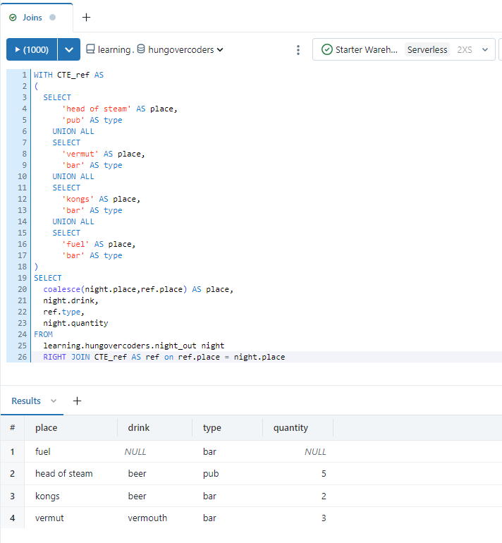
Right Join

If we run the following command we will get four results returned. The right join means that rows that exist in the right hand table will always be returned even if the row does not exist in the right hand table. In this case “drink”, “place” and “quantity” is NULL for Fuel because it does not exist in the left hand night out data table. We have ensured the name of the place is still brought back by placing a coalesce in the statement that will enter the data in the return statement from the left or right side of the join, depending on where it exists.

WITH CTE_ref AS
(
  SELECT
      'head of steam' AS place,
      'pub' AS type
    UNION ALL
    SELECT
      'vermut' AS place,
      'bar' AS type
    UNION ALL
    SELECT
      'kongs' AS place,
      'bar' AS type
    UNION ALL
    SELECT
      'fuel' AS place,
      'bar' AS type
)
SELECT
  coalesce(night.place,ref.place) AS place,
  night.drink,
  ref.type,
  night.quantity
FROM
  learning.hungovercoders.night_out night
  RIGHT JOIN CTE_ref AS ref on ref.place = night.place

Aggregations and Group by

Create a query and name it “Aggregations”, saving in the lrn_sql_analyst location. Lets first perform aggregations against the whole night out table by executing the following

SELECT
  COUNT(*) AS CountOfRows,
  SUM(quantity) AS DrinksDrunk,
  MAX(quantity) AS MaxDrinksDrunkInOneLocation,
  MIN(quantity) AS MinDrinksDrunkInOneLocation
FROM
  learning.hungovercoders.night_out;

• COUNT will give us the number of rows in the table.
• SUM of quantity will give us the total drinks drunk.
• MAX of quantity will give us the maximum drinks drunk in a location.
• MIN of quantity will give us the minimum drinks drunk in a location.

Now lets add a group by to get the same for the different types of drinks.

SELECT
  drink,
  COUNT(*) AS CountOfRows,
  SUM(quantity) AS DrinksDrunk,
  MAX(quantity) AS MaxDrinksDrunkInOneLocation,
  MIN(quantity) AS MinDrinksDrunkInOneLocation
FROM
  learning.hungovercoders.night_out
  GROUP BY drink;

Now lets add a rollup to the drink group by which will also give us the cross section of our group by properties, in this case just the total.

SELECT
  drink,
  COUNT(*) AS CountOfRows,
  SUM(quantity) AS DrinksDrunk,
  MAX(quantity) AS MaxDrinksDrunkInOneLocation,
  MIN(quantity) AS MinDrinksDrunkInOneLocation
FROM
  learning.hungovercoders.night_out
  GROUP BY drink WITH ROLLUP;

Lets try a grouping set for drink and place. This will just give the totals for drink and place, not providing the cross sections.

SELECT
  drink,
  place,
  COUNT(*) AS CountOfRows,
  SUM(quantity) AS DrinksDrunk,
  MAX(quantity) AS MaxDrinksDrunkInOneLocation,
  MIN(quantity) AS MinDrinksDrunkInOneLocation
FROM
  learning.hungovercoders.night_out
  GROUP BY  GROUPING SETS (drink, place)
  ORDER BY drink, place;

Now lets add a cube to the group by. This will give us the cross section of every combination of drink and place, including their totals, and the grand total!

SELECT
  drink,
  place,
  COUNT(*) AS CountOfRows,
  SUM(quantity) AS DrinksDrunk,
  MAX(quantity) AS MaxDrinksDrunkInOneLocation,
  MIN(quantity) AS MinDrinksDrunkInOneLocation
FROM
  learning.hungovercoders.night_out
  GROUP BY drink, place WITH CUBE
  ORDER BY drink, place;

Transform Arrays

Create a new query called “Transform Arrays”, saving in the lrn_sql_analyst location and we’ll do some basic array queries you’ll want to know about.

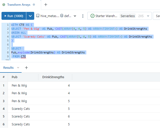
If we want to convert an array into rows we can use the explode command.

WITH CTE AS (
SELECT 'Pen & Wig' AS Pub, CAST(ARRAY(4, 4, 5) AS ARRAY<TINYINT>) AS DrinkStrengths
UNION ALL
SELECT 'Scaredy Cats' AS Pub, CAST(ARRAY(5, 6, 5) AS ARRAY<TINYINT>) AS DrinkStrengths
)

SELECT
Pub,explode(DrinkStrengths) AS DrinkStrengths
 FROM CTE

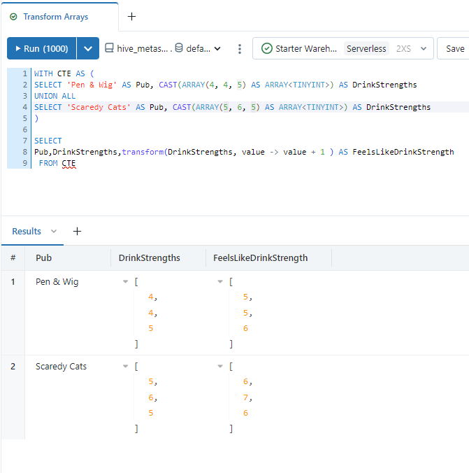
If we want to perform calculations on items within an array we can use TRANSFORM.

WITH CTE AS (
SELECT 'Pen & Wig' AS Pub, CAST(ARRAY(4, 4, 5) AS ARRAY<TINYINT>) AS DrinkStrengths
UNION ALL
SELECT 'Scaredy Cats' AS Pub, CAST(ARRAY(5, 6, 5) AS ARRAY<TINYINT>) AS DrinkStrengths
)

SELECT
Pub,DrinkStrengths,transform(DrinkStrengths, value -> value + 1 ) AS FeelsLikeDrinkStrength
 FROM CTE

In this case we can see we have added one to each value in the array to get a more accurate “feels like drink strength” value.

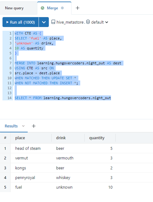
Merge

Create a new query called “Merge”, saving in the lrn_sql_analyst location. We can use the MERGE statement to:

• Insert if the source data does not match data already in the destination table.
• Delete if the destination data does match incoming source data.
• Update if the key field is in both tables but the other attributes have different tables.

Enter this SQL in your new query and execute. This will add the last place of the night out we forgot about with some unknown details.

WITH CTE AS (
SELECT 'fuel' AS place,
'unknown' AS drink,
10 AS quantity
)

MERGE INTO learning.hungovercoders.night_out AS dest
USING CTE AS src ON
src.place = dest.place
WHEN MATCHED THEN UPDATE SET *
WHEN NOT MATCHED THEN INSERT *;


SELECT * FROM learning.hungovercoders.night_out

Query History

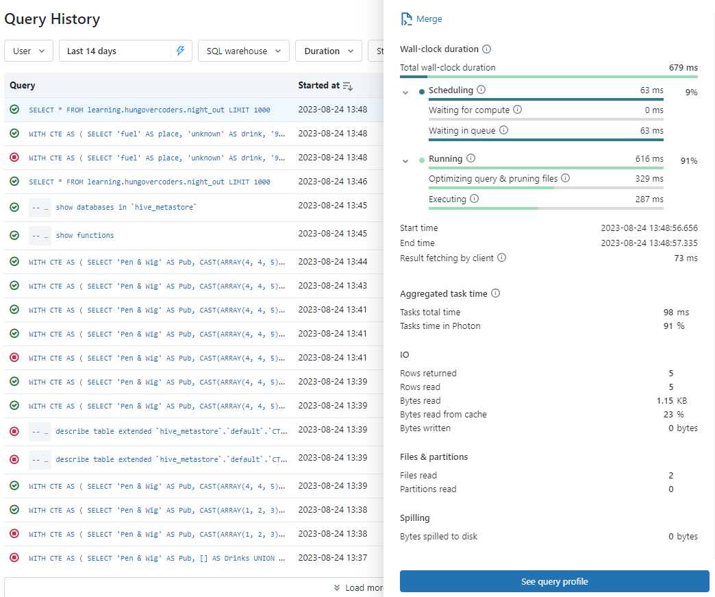
Now that we have a load of queries we have been running, lets look at the query history on the left hand side of the workspace.

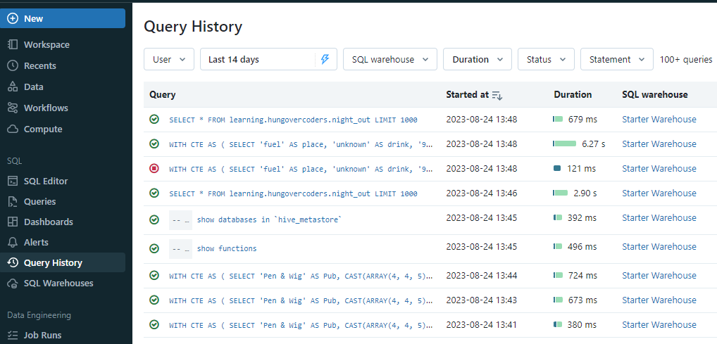
This shows all the queries that have been executed over the time range selected, how long they ran for, the SQL warehouse used and the user. If you select one of the queries you get further details that can help you debug and understand things like if the cache was used in the IO section.

Visualisations

Go back to SQL editor and create a new query called “Visualisations”, saving it in the lrn_sql_analyst folder. Enter the following query which we will…

• Add a weeks worth of dates so we can look at some time based visuals.
• Add a random value between the range of -2 and 2 to make the data a bit more changeable.
• Add a total aggregation for all the data using grouping sets.
• Add a target column.
• Excluded fuel as its a crazy high number.

WITH CTE_dt AS (
  SELECT current_date() AS Dt
  UNION ALL
  SELECT current_date() - INTERVAL 1 DAYS AS Dt
  UNION ALL
    SELECT current_date() - INTERVAL 2 DAYS AS Dt
  UNION ALL
    SELECT current_date() - INTERVAL 3 DAYS AS Dt
  UNION ALL
    SELECT current_date() - INTERVAL 4 DAYS AS Dt
  UNION ALL
    SELECT current_date() - INTERVAL 5 DAYS AS Dt
  UNION ALL
    SELECT current_date() - INTERVAL 6 DAYS AS Dt
)
, CTE_base AS (
SELECT
dt, place, drink, quantity + floor(rand()*2) + -2 AS quantity
FROM learning.hungovercoders.night_out
CROSS JOIN CTE_dt
)

SELECT dt, place, drink, SUM(quantity) AS Quantity, SUM(quantity)+1 AS Target
FROM CTE_base
GROUP BY  GROUPING SETS ((dt, place, drink), ())
ORDER BY dt, place, drink;

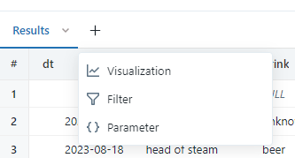
First add a visualisation by clicking the plus next to the results and choose Visualisation.

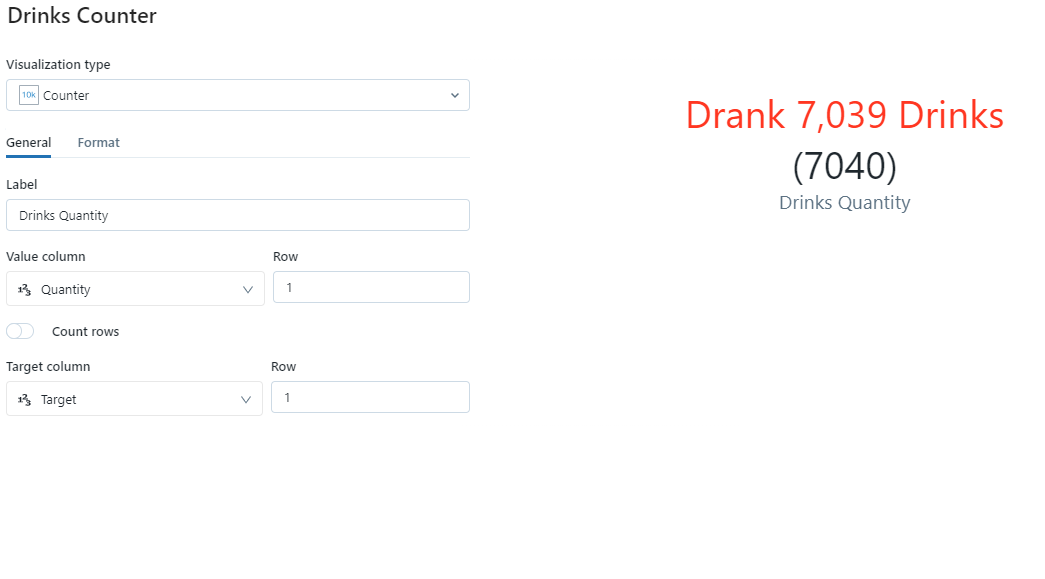
• Choose visualisation type of counter.
• Name it “Drinks Counter”.
• Set the label to be drinks quantity.
• Set the value volume to be quantity and the row this is contained in to be 1. This will use the total column we have created using the grouping sets command and ensured will be row 1 using the order by.
• Set the target column to be target and also have this in row 1. We will see that the counter value will show red as its below target! If this was above target it would be green.
• Explore the format tab and add “Drank” as the formatting string prefix and set the suffix to be “ Drinks”.
• Then save.

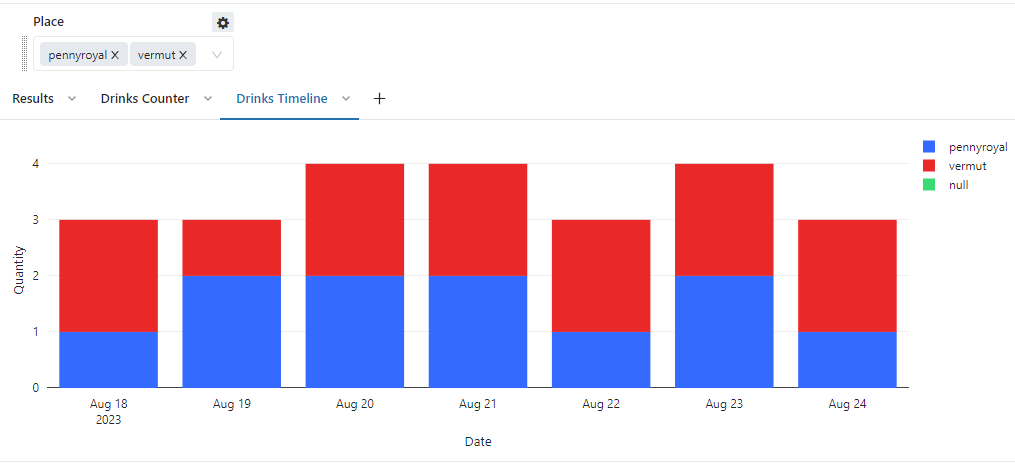
Now add another visualisation by clicking the plus next to the results and choose Visualisation.

• Choose visualisation type of bar.
• Name it “Drinks Timeline”.
• Set the x column to be dt.
• Set the y column to be quantity.
• Set the group by to be place.
• Set stacking to be Stack.
• In the x axis section set the name to be Date.
• In the y axis section set the name to be Quantity.
• Then save.

These are just two of the example visualisations and I recommend checking them all out and having a bit of a play…

Parameters

We can add parameters to our queries using the syntax. These parameters can be freetext, manually entered dropdowns, dates, or dropdowns from a query, which we are going to use here.

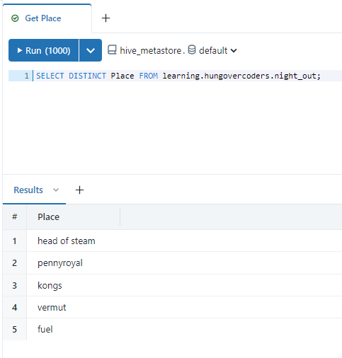
First lets create a query we can use in a dropdown list that can feed the parameter to make it nice and usable. Create a new query called “Get Place” and save it in lrn_data_analyst. Enter the following query and save it.

SELECT DISTINCT Place FROM learning.hungovercoders.night_out;

In our previous “Visualisations” query lets add a place parameter to it. Replace your visualisations query with the following, noting the parameter for place that now exists in the where clause. We are using IN as its going to be a multi select parameter. The “place IS NULL” part of the where clause is to ensure we always return the total as well.

WITH CTE_dt AS (
  SELECT current_date() AS Dt
  UNION ALL
  SELECT current_date() - INTERVAL 1 DAYS AS Dt
  UNION ALL
    SELECT current_date() - INTERVAL 2 DAYS AS Dt
  UNION ALL
    SELECT current_date() - INTERVAL 3 DAYS AS Dt
  UNION ALL
    SELECT current_date() - INTERVAL 4 DAYS AS Dt
  UNION ALL
    SELECT current_date() - INTERVAL 5 DAYS AS Dt
  UNION ALL
    SELECT current_date() - INTERVAL 6 DAYS AS Dt
)
, CTE_base AS (
SELECT
dt, place, drink, quantity + floor(rand()*2) + -2 AS quantity
FROM learning.hungovercoders.night_out
CROSS JOIN CTE_dt
WHERE place IS NULL OR place IN ({{ place }})
)

SELECT dt, place, drink, SUM(quantity) AS Quantity, SUM(quantity)+1 AS Target
FROM CTE_base
GROUP BY  GROUPING SETS ((dt, place, drink), ())
ORDER BY dt, place, drink;

You will see at the bottom of the query as soon as you enter the parameters that boxes will appear to represent them.

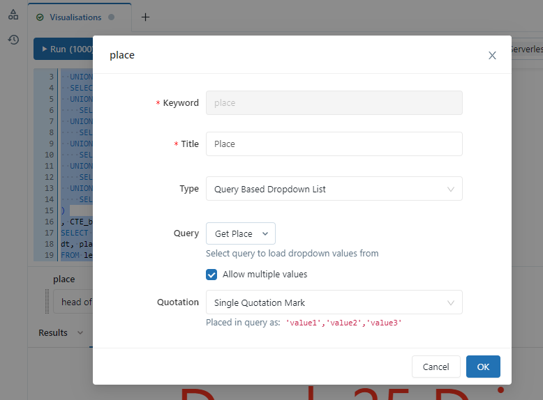
• Click the little settings cog.
• Set the title as Place.
• Set the type to be “Query Based Dropdown List”.
• Set the Query to be “Get Place”.
• Tick the allow multiple values box.

We can now choose the places we want to query very easily from the dropdown that is populated for us as a parameter.

Dashboard

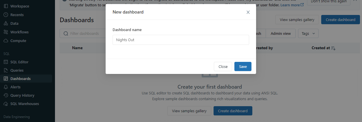
Navigate to dashboard on the left hand side of the workspace. Click create dashboard and name it “Nights Out”.

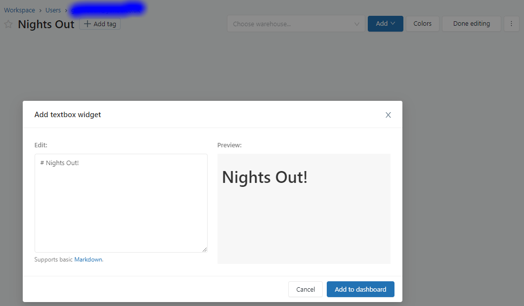
Add a text box and as its markdown simply enter

# Nights Out!

Next…

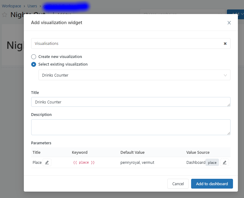
• Add a visualisation by selecting the “Visualisations” query and choosing “Drinks Counter” from selecting existing visualisation.
• Change the title to be “Drinks Counter”.
• Leave the parameter as place and note the value source will be a new dashboard parameter. This will be created for us and should work on the next visualisation we add as well.

Next…

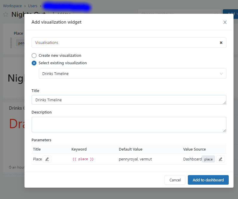
• Add another visualisation by selecting the “Visualisations” query and choosing “Drinks Timeline” from selecting existing visualisation.
• Change the title to be “Drinks Timeline”.
• Leave the parameter as place and note the value source will be a new dashboard parameter. This should reuse the same one from before so the dashboard parameter applies to all visualisations.

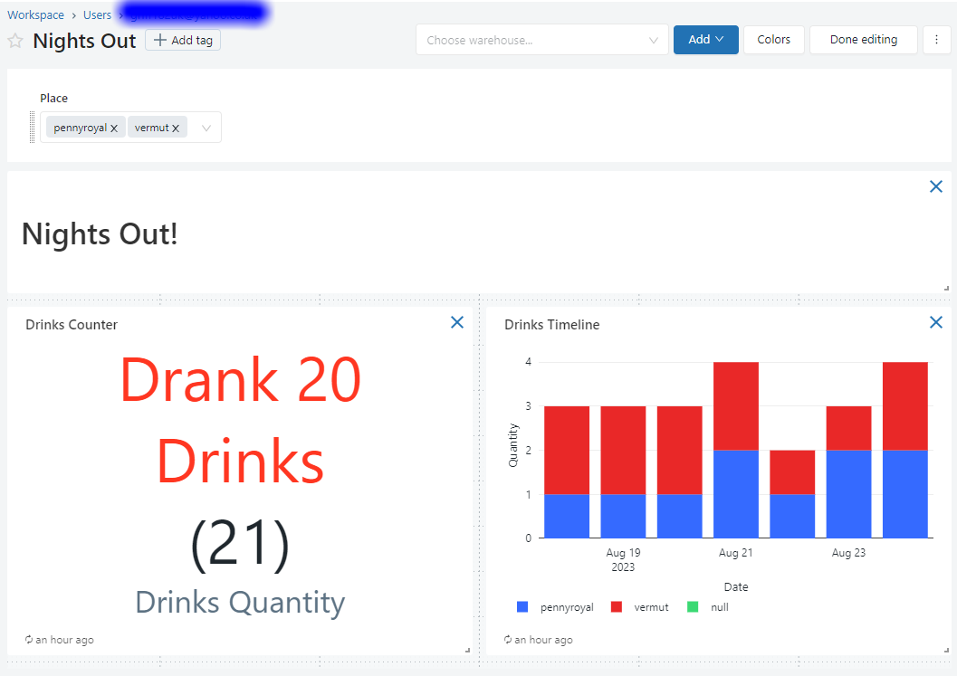
Shuffle your dashboard about a bit and you should end up with something like the below.

• Nicely formatted.
• Markdown text describing the dashboard.
• Global parameter that affects all visualisations.
• Multiple visualisations.

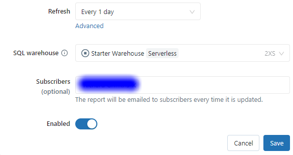
You can schedule the dashboard to run at a cadence you wish and also send the output to relevant subscribers by going to “Schedule” and setting the relevant options. Ensure you use an appropriately sized SQL Warehouse and don’t run it too often as it will likely never go off and you will incur costs! For the testing I would just leave it as never.

Alerts

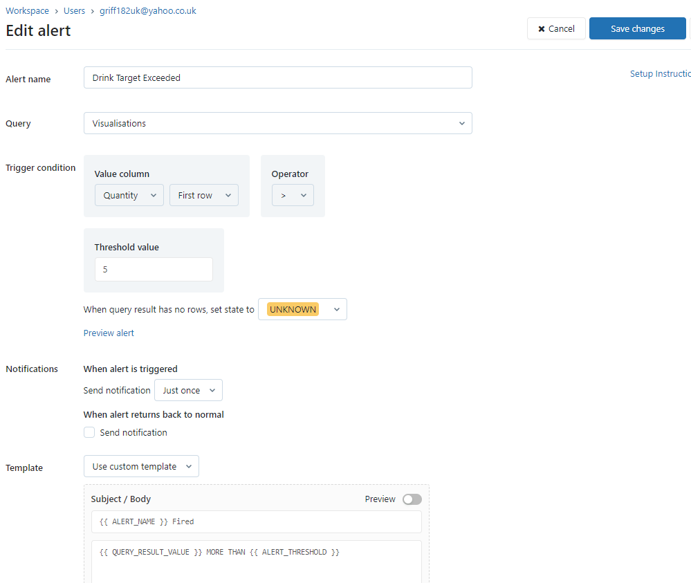
Navigate to alerts on the left hand side of the workspace and select create alert. Alerts allow you to react to certain conditions. Setup the alert as follows:

• Set the alert name to be Drink Target Exceeded.
• Set the Query to be Visualisations.
• Set the Value column to be Quantity and in the first row.
• Set the Operator to be More Than (>).
• Set the Threshold Value to be 5.
• Set the send notification to be “Each time alert is evaluated” so that we ensure we can trigger it every time we refresh manually.
• Leave the rest of the defaults but then use a custom template and in the Subject add “{{ ALERT_NAME }} Fired” and in the Body add “{{ QUERY_RESULT_VALUE }} MORE THAN {{ ALERT_THRESHOLD }}” which will add dynamic values from the alert. Tick preview to see the outcome of this.
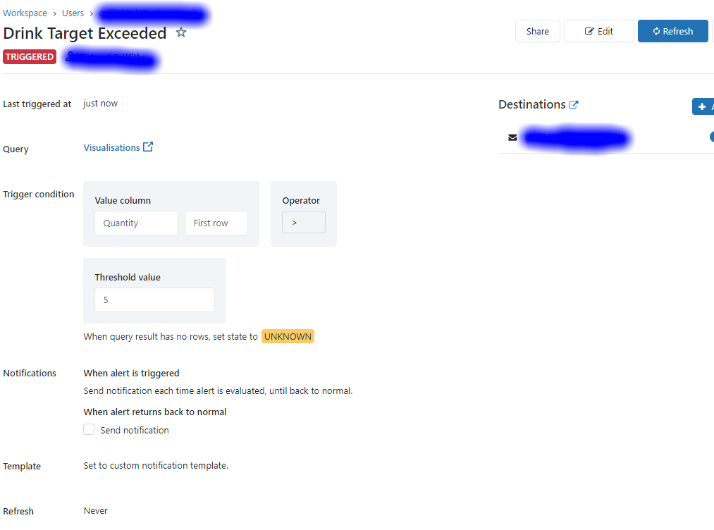
• Leave refresh as never as we will run this manually for now. We can schedule to have it run more often but this would incur costs and as we are just learning we don’t want to do this.
• Save the alert.

Refresh the alert and you should see its status change to triggered. You’ll also get an e-mail with the custom template we specified. You can add more destinations to these alerts in the integrations section of the workspace which include webhooks and slack, as well as email.

Book the Exam

Now that you have queried your night out data its time to head over to Kryterion Certification Login and book that exam. I hope you are soon creating your own night out data in celebration of your exam passing success!

Once you’re done you can also remove the resources you have made if you did make any, or keep them for further practice and just ensure your clusters etc are kept off to reduce costs.